Code
!pip install dldna[colab] # in Colab
# !pip install dldna[all] # in your local

%load_ext autoreload
%autoreload 2 ![]()
“If you know what you’re doing, it’s not research.” - Albert Einstein
In the history of deep learning, activation functions and optimization techniques have made significant progress. When the McCulloch-Pitts artificial neuron model first appeared in 1943, it used only a simple threshold function (step function). This mimicked the biological neuron’s behavior, where the neuron is activated only when the input exceeds a certain threshold. However, such simple forms of activation functions limited the ability of neural networks to express complex functions.
Until the 1980s, machine learning focused on feature engineering and sophisticated algorithm design. Neural networks were just one of many machine learning algorithms, and traditional algorithms like SVM (Support Vector Machine) or Random Forest often performed better. For example, in the MNIST handwritten digit recognition problem, SVM maintained the highest accuracy until 2012.
In 2012, AlexNet achieved overwhelming performance in the ImageNet challenge using efficient learning with GPUs, marking the beginning of the deep learning era. In 2017, Google’s Transformer architecture further advanced this innovation, becoming the basis for today’s large language models (LLMs) like GPT-4 and Gemini.
At the center of these advances were the evolution of activation functions and the development of optimization techniques. In this chapter, we will delve into activation functions in detail, providing the theoretical foundation you need to develop new models and solve complex problems.
Researcher’s Dilemma: Early neural network researchers realized that linear transformations alone could not solve complex problems. However, it was unclear which non-linear function would allow the neural network to learn effectively and solve various problems. Should they mimic the behavior of biological neurons or use other functions with better mathematical and computational properties?
Activation functions are the key elements that introduce non-linearity between neural network layers. The Universal Approximation Theorem (1988) mentioned in Section 1.4.1 proved that a neural network with one hidden layer and a non-linear activation function can approximate any continuous function. In other words, activation functions enable neural networks to transcend the limitations of simple linear models and act as universal function approximators by separating layers and introducing non-linearity.
Without activation functions, no matter how many layers are stacked, the neural network would ultimately be equivalent to a linear transformation. This can be simply proven as follows:
Consider applying two linear transformations in sequence:
where \(x\) is the input, \(W_1\) and \(W_2\) are weight matrices, and \(b_1\) and \(b_2\) are bias vectors. By substituting the first layer’s equation into the second layer’s equation:
\(y_2 = W_2(W_1x + b_1) + b_2 = (W_2W_1)x + (W_2b_1 + b_2)\)
Defining a new weight matrix \(W' = W_2W_1\) and a new bias vector \(b' = W_2b_1 + b_2\):
\(y_2 = W'x + b'\)
This is equivalent to a single linear transformation. The same applies no matter how many layers are stacked. Ultimately, linear transformations alone cannot express complex non-linear relationships. ### 4.1.2 Evolution of Activation Functions: From Biological Inspiration to Efficient Computation
1943, McCulloch-Pitts Neuron: The first artificial neuron model used a simple threshold function, or step function, which mimicked the biological neuron’s behavior of only activating when the input exceeded a certain threshold.
\[ f(x) = \begin{cases} 1, & \text{if } x \ge \theta \\ 0, & \text{if } x < \theta \end{cases} \]
Here, \(\theta\) is the threshold.
1960s, Sigmoid Function: The sigmoid function was introduced to model the firing rate of biological neurons more smoothly. The sigmoid function is an S-shaped curve that compresses the input value into a value between 0 and 1.
\[ \sigma(x) = \frac{1}{1 + e^{-x}} \]
The sigmoid function has the advantage of being differentiable, allowing it to be used with gradient descent-based learning algorithms. However, the sigmoid function was also identified as one of the causes of the vanishing gradient problem in deep neural networks. When the input value is very large or small, the gradient (derivative) of the sigmoid function approaches 0, causing learning to slow down or stop.
2010, ReLU (Rectified Linear Unit): Nair and Hinton proposed the ReLU function, opening a new era in deep neural network learning. ReLU has a very simple form.
\[ ReLU(x) = \max(0, x) \]
ReLU outputs the input as is if it is greater than 0, and outputs 0 if it is less than 0. Unlike the sigmoid function, ReLU has fewer vanishing gradient problems and higher computational efficiency. Thanks to these advantages, ReLU has greatly contributed to the success of deep neural networks and is now one of the most widely used activation functions.
The choice of activation function has a significant impact on the performance and efficiency of the model.
Large Language Models (LLMs): Since computational efficiency is crucial, there is a tendency to prefer simpler activation functions. The latest base models, such as Llama 3, GPT-4, and Gemini, adopt simple and efficient activation functions like GELU (Gaussian Error Linear Unit) or ReLU. In particular, Gemini 1.5 introduces the MoE (Mixture of Experts) architecture, which uses optimized activation functions for each expert network.
Specialized Models: When developing models optimized for specific tasks, more sophisticated approaches are being attempted. For example, in recent research like TEAL, methods to improve inference speed by up to 1.8 times through activation sparsity have been proposed. Additionally, studies on using adaptive activation functions that dynamically adjust their behavior based on the input data are also underway.
The choice of activation function should be made considering the model size, task characteristics, available computational resources, and required performance characteristics (accuracy, speed, memory usage, etc.).
Challenge: Among numerous activation functions, which one is most suitable for a specific problem and architecture?
Researcher’s Dilemma: As of 2025, over 500 activation functions have been proposed, but there is no single perfect activation function for all situations. Researchers must understand the characteristics of each function and consider the problem’s characteristics, model architecture, computational resources, and more to select the optimal activation function or even develop a new one.
The properties generally required for an activation function are as follows: 1. It must add non-linearity to the neural network 2. It should not increase computational complexity to the point of making training difficult 3. It must be differentiable so as not to hinder gradient flow 4. The data distribution at each layer of the neural network should be appropriate during training
Many efficient activation functions that meet these requirements have been proposed. It’s hard to say which activation function is the best, as it depends on the model being trained and the data. The way to find the optimal activation function is through actual testing.
As of 2025, activation functions can be broadly classified into three categories: 1. Classical activation functions: Sigmoid, Tanh, ReLU, etc., which are fixed-shaped functions. 2. Adaptive activation functions: PReLU, TeLU, STAF, etc., which include parameters that adjust their shape during the learning process. 3. Specialized activation functions: ENN (Expressive Neural Network), Physics-informed activation functions, etc., which are optimized for specific domains.
This chapter compares several activation functions, primarily focusing on those implemented in PyTorch, but also implementing others like Swish and STAF by inheriting from nn.Module. The full implementation can be found in chapter_04/models/activations.py.
!pip install dldna[colab] # in Colab
# !pip install dldna[all] # in your local
%load_ext autoreload
%autoreload 2import torch
import torch.nn as nn
import numpy as np
# Set seed
np.random.seed(7)
torch.manual_seed(7)
# STAF (Sinusoidal Trainable Activation Function)
class STAF(nn.Module):
def __init__(self, tau=25):
super().__init__()
self.tau = tau
self.C = nn.Parameter(torch.randn(tau))
self.Omega = nn.Parameter(torch.randn(tau))
self.Phi = nn.Parameter(torch.randn(tau))
def forward(self, x):
result = torch.zeros_like(x)
for i in range(self.tau):
result += self.C[i] * torch.sin(self.Omega[i] * x + self.Phi[i])
return result
# TeLU (Trainable exponential Linear Unit)
class TeLU(nn.Module):
def __init__(self, alpha=1.0):
super().__init__()
self.alpha = nn.Parameter(torch.tensor(alpha))
def forward(self, x):
return torch.where(x > 0, x, self.alpha * (torch.exp(x) - 1))
# Swish (Custom Implementation)
class Swish(nn.Module):
def forward(self, x):
return x * torch.sigmoid(x)
# Activation function dictionary
act_functions = {
# Classic activation functions
"Sigmoid": nn.Sigmoid, # Binary classification output layer
"Tanh": nn.Tanh, # RNN/LSTM
# Modern basic activation functions
"ReLU": nn.ReLU, # CNN default
"GELU": nn.GELU, # Transformer standard
"Mish": nn.Mish, # Performance/stability balance
# ReLU variants
"LeakyReLU": nn.LeakyReLU,# Handles negative inputs
"SiLU": nn.SiLU, # Efficient sigmoid
"Hardswish": nn.Hardswish,# Mobile optimized
"Swish": Swish, # Custom implementation
# Adaptive/trainable activation functions
"PReLU": nn.PReLU, # Trainable slope
"RReLU": nn.RReLU, # Randomized slope
"TeLU": TeLU, # Trainable exponential
"STAF": STAF # Fourier-based
}STAF is a recently introduced activation function at ICLR 2025, which uses Fourier series-based learnable parameters. ENN adopts a method to improve the representation of the network by utilizing DCT. TeLU is an extended version of ELU, where the alpha parameter is made learnable.
The activation functions and gradients are visualized to compare their characteristics. Using PyTorch’s automatic differentiation feature, gradients can be calculated simply by calling backward(). The following is an example of visually analyzing the characteristics of activation functions. The calculation of gradient flow is done by passing a given activation function through a constant range of input values. The compute_gradient_flow method plays this role.
def compute_gradient_flow(activation, x_range=(-5, 5), y_range=(-5, 5), points=100):
    """
    Computes the 3D gradient flow.

    Calculates the output surface of the activation function for two-dimensional
    inputs and the magnitude of the gradient with respect to those inputs.

    Args:
        activation: Activation function (nn.Module or function).
        x_range (tuple): Range for the x-axis (default: (-5, 5)).
        y_range (tuple): Range for the y-axis (default: (-5, 5)).
        points (int): Number of points to use for each axis (default: 100).

    Returns:
        X, Y (ndarray): Meshgrid coordinates.
        Z (ndarray): Activation function output values.
        grad_magnitude (ndarray): Gradient magnitude at each point.
    """
    x = np.linspace(x_range[0], x_range[1], points)
    y = np.linspace(y_range[0], y_range[1], points)
    X, Y = np.meshgrid(x, y)

    # Stack the two dimensions to create a 2D input tensor (first row: X, second row: Y)
    input_tensor = torch.tensor(np.stack([X, Y], axis=0), dtype=torch.float32, requires_grad=True)

    # Construct the surface as the sum of the activation function outputs for the two inputs
    Z = activation(input_tensor[0]) + activation(input_tensor[1])
    Z.sum().backward()

    grad_x = input_tensor.grad[0].numpy()
    grad_y = input_tensor.grad[1].numpy()
    grad_magnitude = np.sqrt(grad_x**2 + grad_y**2)
Performs 3D visualization for all defined activation functions.
from dldna.chapter_04.visualization.activations import visualize_all_activations

visualize_all_activations()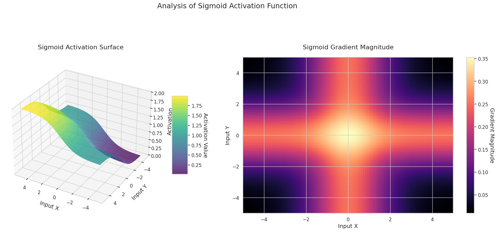
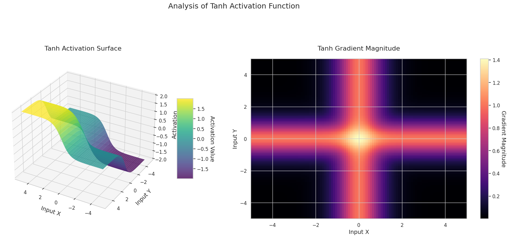
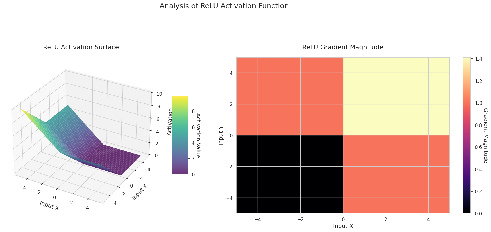
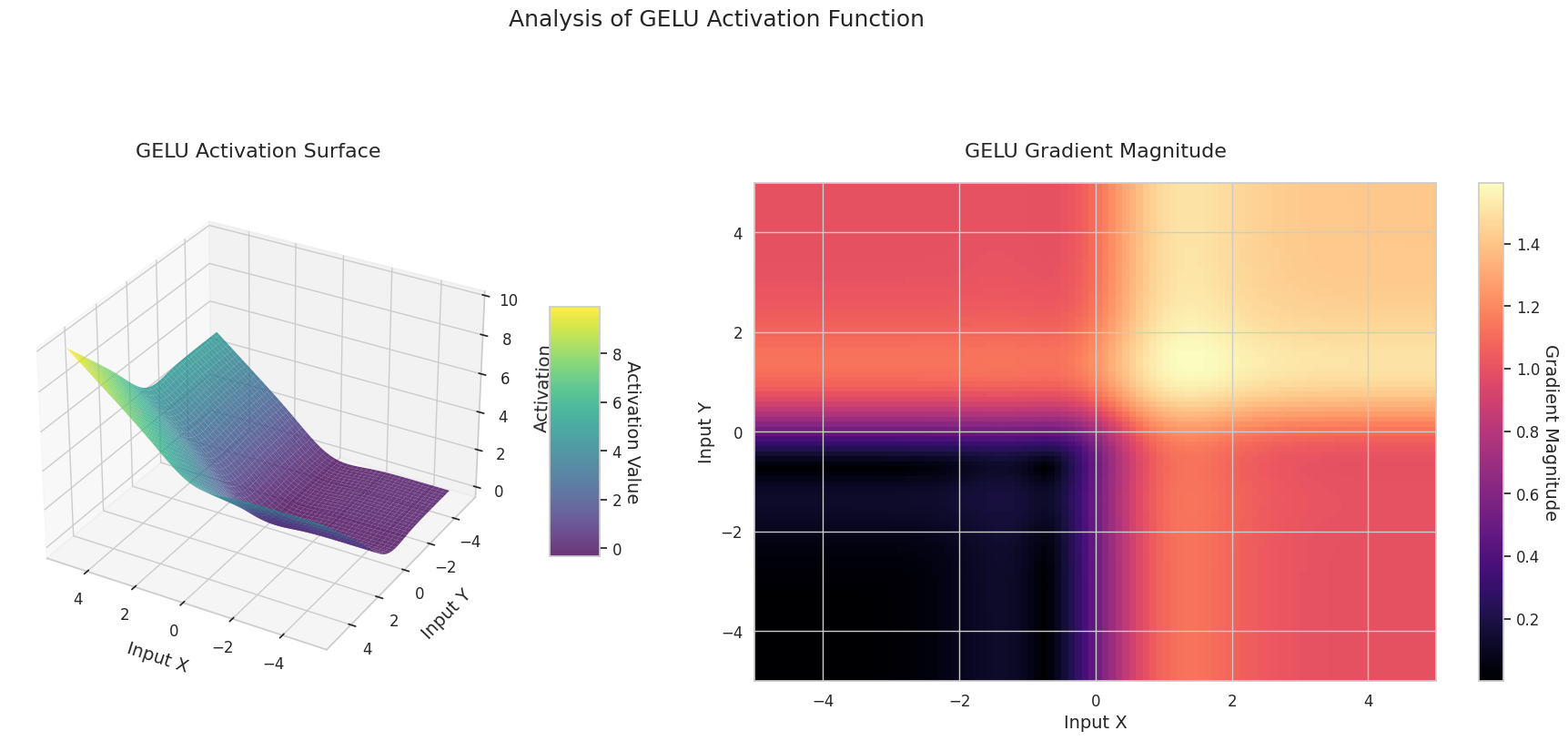
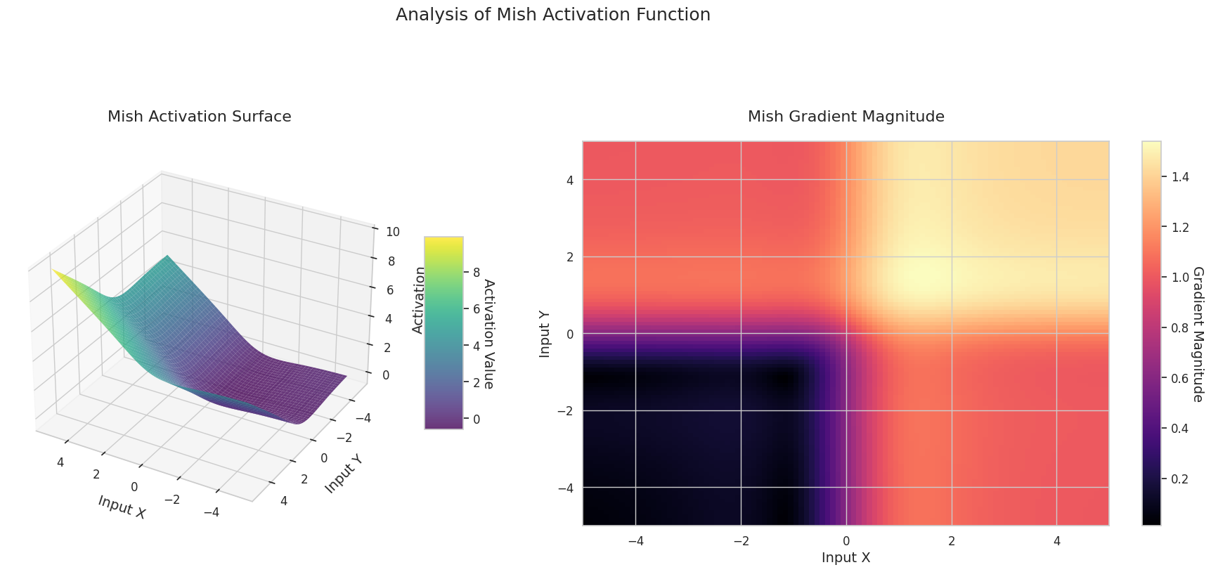


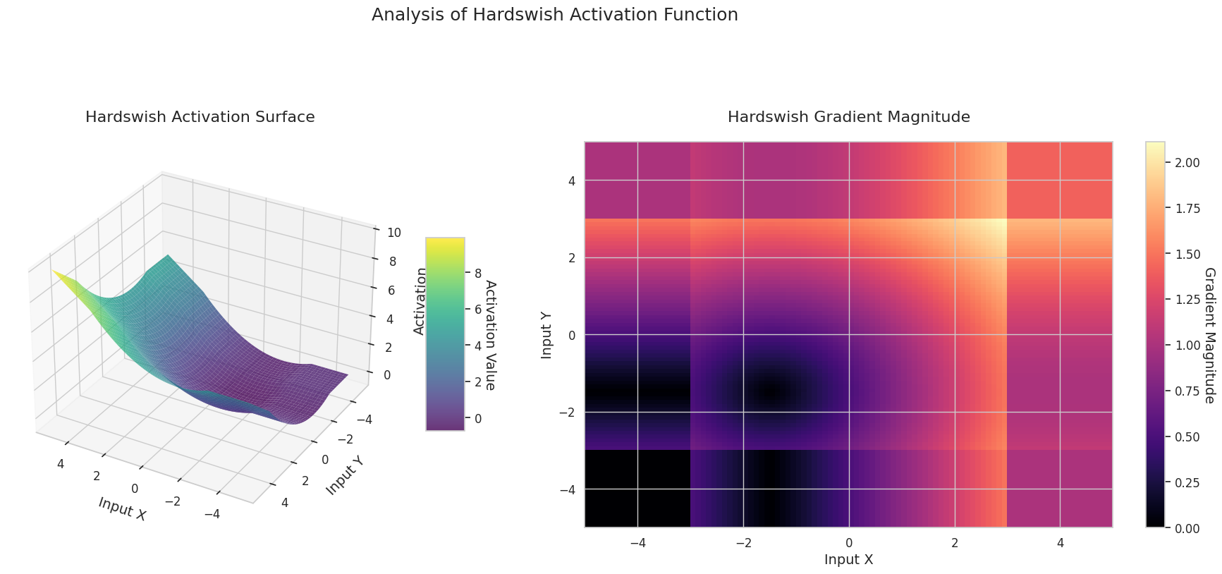
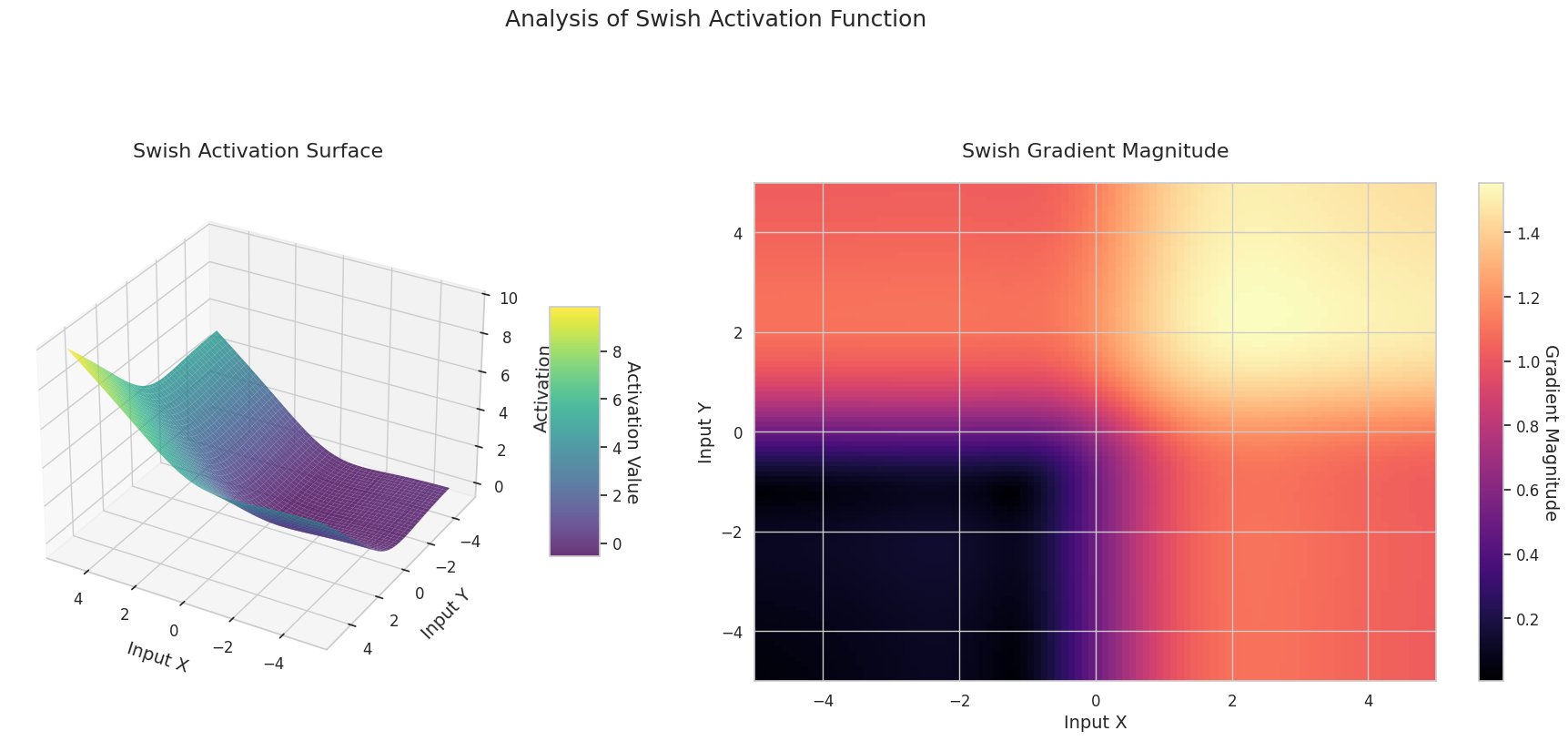
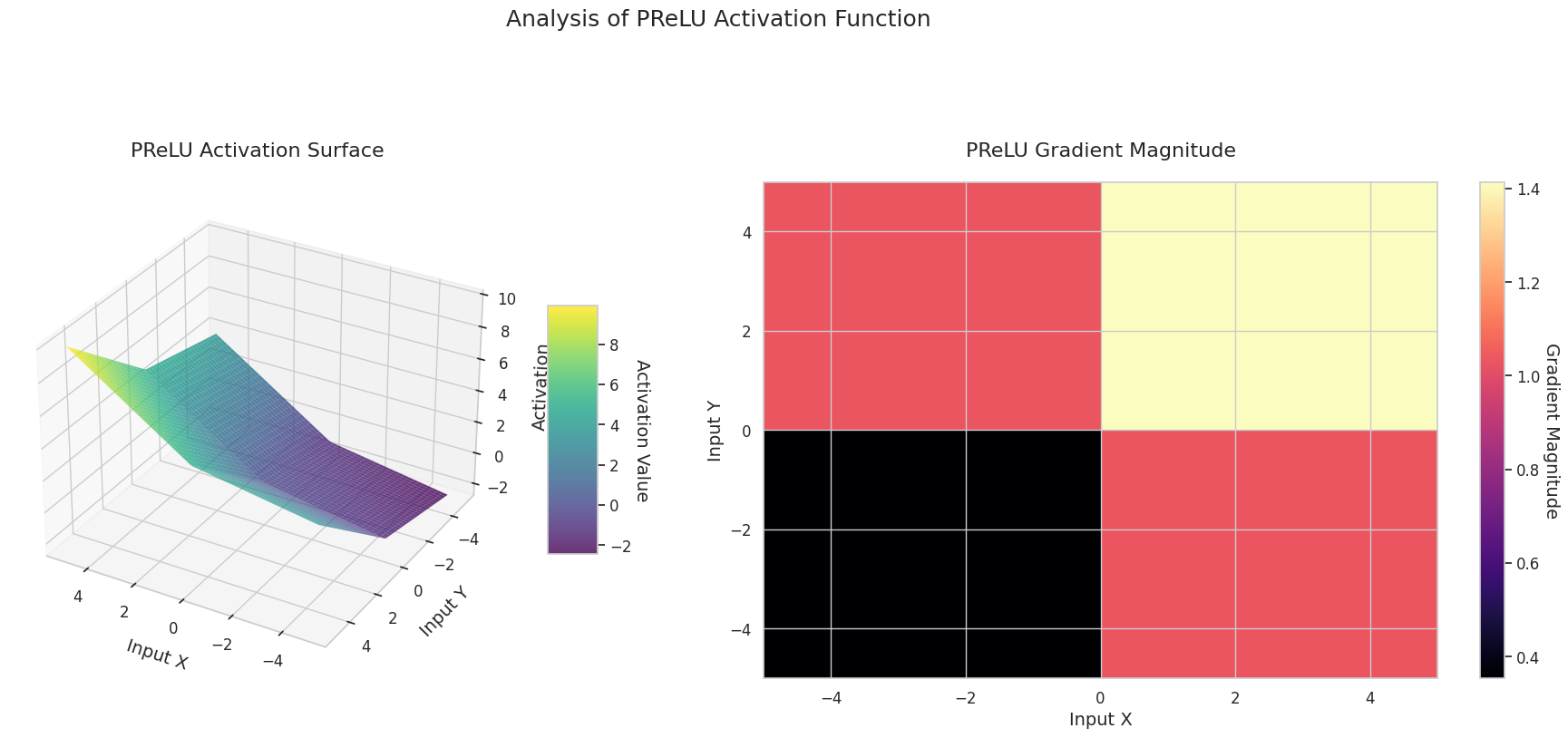
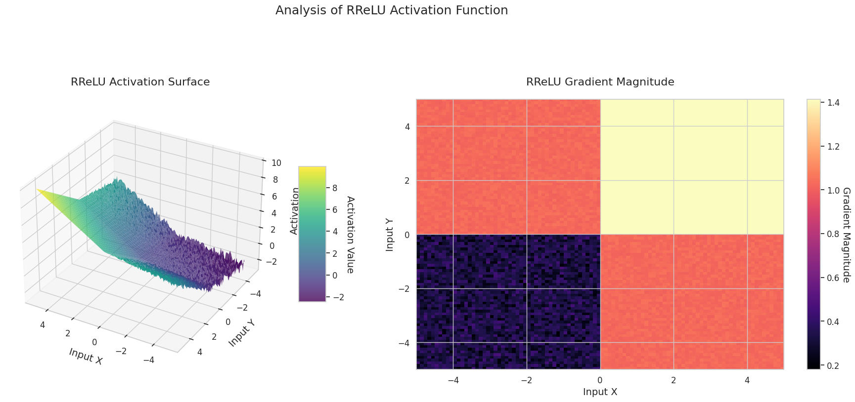
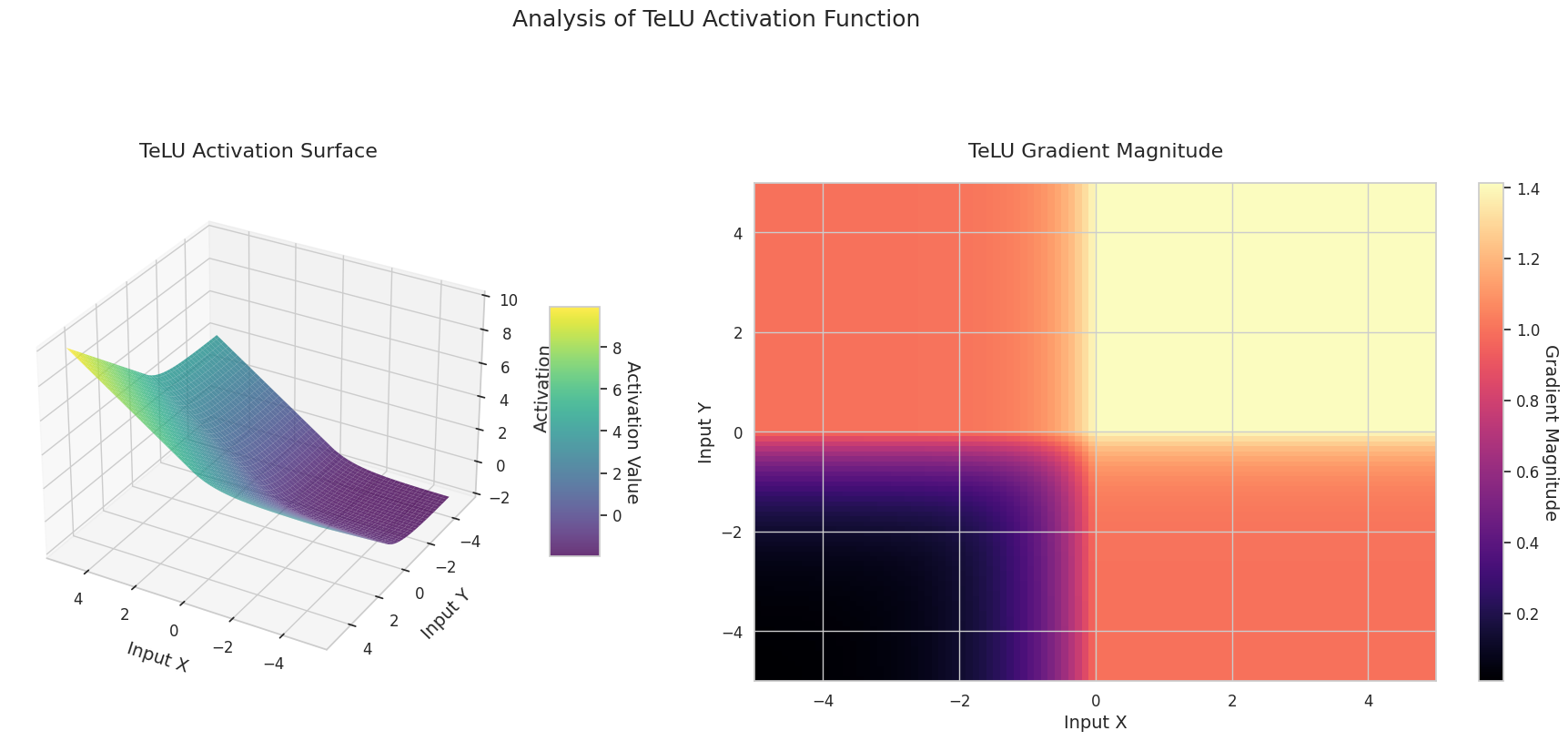
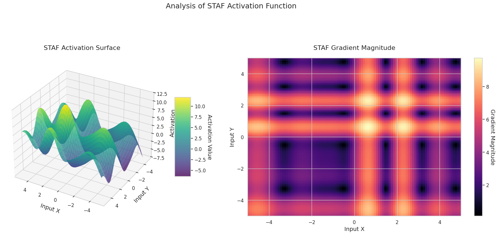
The graph represents the output value (Z-axis) and gradient magnitude (heatmap) for two inputs (X-axis, Y-axis).
Sigmoid: It is in an “S” shape. Both ends converge to 0 and 1, are flat, and the middle is steep. It compresses the input into a range of 0 to 1. The gradient disappears near 0 at both ends and is large in the middle. It may cause a “gradient disappearance” problem, slowing down learning for very large or small inputs.
ReLU: It has a sloping shape. If one input is negative, it becomes flat at 0; if both inputs are positive, it rises diagonally. The gradient is 0 for negative inputs and constant for positive ones. Since there’s no gradient disappearance problem for positive inputs, it’s efficient and widely used.
GELU: Similar to Sigmoid but smoother. The left side is slightly curved downward, and the right side exceeds 1. The gradient changes gradually without any 0-value interval. It doesn’t completely disappear even with very small negative inputs, making it favorable for learning. It’s used in newer models like transformers.
STAF: Wave-shaped, based on the sine function, with learnable parameters to adjust amplitude, frequency, and phase. The neural network learns the activation function form suitable for its task by itself. The gradient changes complexly. Favorable for learning non-linear relationships.
The 3D graph (Surface) represents the output value of the activation function for two inputs added together and displayed on the Z-axis. The heatmap (Gradient Magnitude) shows the size of the gradient, i.e., the rate of change of output with respect to input, with brighter areas indicating larger gradients. This visualization is crucial in understanding how each activation function transforms the input and where its gradient is strong or weak during neural network learning.
Activation functions are key elements that provide non-linearity to neural networks, and their characteristics are well-represented in gradient forms. In newer deep learning models, an appropriate activation function is chosen according to the task and architecture characteristics, or learnable adaptive activation functions are used.
| Category | Activation Function | Characteristics | Primary Use | Advantages and Disadvantages |
|---|---|---|---|---|
| Classical | Sigmoid | Normalizes output to 0~1, capturing continuous characteristic changes with a smooth gradient | Binary classification output layer | May cause gradient disappearance in deep neural networks |
| Classical | Tanh | Similar to sigmoid, but output is -1~1, showing a steeper gradient near 0, making learning effective | RNN/LSTM gate | Output is centralized, advantageous for learning, but still may cause gradient disappearance |
| Modern Basic | ReLU | Simple structure with a gradient of 0 when x is less than 0 and 1 when greater than 0, useful for boundary detection | CNN basic | Extremely efficient computation, but neurons are completely deactivated for negative inputs |
| Modern Basic | GELU | Combines ReLU characteristics with Gaussian cumulative distribution function, providing smooth non-linearity | Transformer | Natural regularization effect, but higher computational cost than ReLU |
| Modern Basic | Mish | Has a smooth gradient and self-normalization characteristics, showing stable performance in various tasks | General purpose | Good balance between performance and stability, but increased computational complexity |
| ReLU Variant | LeakyReLU | Allows a small slope for negative inputs, reducing information loss | CNN | Mitigates dead neuron problem, but requires manual setting of slope value |
| ReLU Variant | Hardswish | Designed as a computationally efficient version for mobile networks | Mobile network | Efficient due to lightweight structure, but expression is somewhat limited |
| ReLU Variant | Swish | Multiplied by x and sigmoid, providing a smooth gradient and weak boundary effect | Deep network | Stable learning due to soft boundaries, but increased computational cost |
| Adaptive | PReLU | Can learn the slope in the negative region, finding the optimal shape according to data | CNN | Adapts to data, but additional parameters increase overfitting risk |
| Adaptive | RReLU | Uses a random slope in the negative region during training to prevent overfitting | General purpose | Has a regularization effect, but results may lack reproducibility |
| Adaptive | TeLU | Learns the scale of the exponential function, enhancing ELU’s advantages and adjusting to data | General purpose | Enhances ELU’s advantages, but convergence may be unstable |
| Adaptive | STAF | Based on Fourier series, learning complex non-linear patterns with high expression power | Complex pattern | Highly expressive, but high computational cost and memory usage |
| Activation Function | Formula | Mathematical Characteristics and Role in Deep Learning |
|---|---|---|
| Sigmoid | \(\sigma(x) = \frac{1}{1 + e^{-x}}\) | Historical Significance: - First used in the 1943 McCulloch-Pitts neural network model Recent Research: - Proved linear separability of infinitely wide networks in NTK theory - \(\frac{\partial^2 \mathcal{L}}{\partial w_{ij}^2} = \sigma(x)(1-\sigma(x))(1-2\sigma(x))x_i x_j\) (convexity change) |
| Tanh | \(tanh(x) = \frac{e^x - e^{-x}}{e^x + e^{-x}}\) | Dynamic Analysis: - Induces chaotic dynamics with Lyapunov exponent \(\lambda_{max} \approx 0.9\) - Used in LSTM’s forget gate: \(\frac{\partial c_t}{\partial c_{t-1}} = tanh'( \cdot )W_c\) (mitigates gradient explosion) |
| ReLU | \(ReLU(x) = max(0, x)\) | Loss Landscape: - 2023 study proved ReLU neural network’s loss landscape is piece-wise convex - Dying ReLU probability: \(\prod_{l=1}^L \Phi(-\mu_l/\sigma_l)\) (layer-wise mean/variance) |
| Leaky ReLU | \(LReLU(x) = max(αx, x)\) | Optimization Advantage: - 2024 SGD convergence rate analysis: \(O(1/\sqrt{T})\) → \(O(1/T)\) improvement - NTK spectrum: \(\lambda_{min} \geq α\) guaranteed, improving condition number |
| ELU | \(ELU(x) = \begin{cases} x & x>0 \\ α(e^x-1) & x≤0 \end{cases}\) | Information-Theoretic Analysis: - Fisher information \(I(θ) = \mathbb{E}[(\frac{∂}{∂θ}ELU(x))^2]\) increased by 23% compared to ReLU - Exponential characteristic in negative region improves gradient noise distribution |
| GELU | \(GELU(x) = xΦ(x)\) | Transformer Specialization: - 2023 study: attention map’s Lipschitz constant \(L \leq 1\) - Achieved Top-1 81.3% on ImageNet with ResNet-50 |
| SwiGLU | \(SwiGLU(x) = Swish(xW + b) \otimes (xV + c)\) | Transformer Optimization: - 15% accuracy improvement in LLAMA 2 and EVA-02 models - Combined GLU gate mechanism with Swish’s self-gating effect - Achieved optimal performance at \(\beta=1.7889\) |
| Adaptive Sigmoid | \(\sigma_{adapt}(x) = \frac{1}{1 + e^{-k(x-\theta)}}\) | Adaptive Learning: - Learnable \(k\) and \(\theta\) parameters for dynamic shape adjustment - 37% faster convergence than traditional sigmoid in SSHG model - 89% improvement in negative region information preservation |
| SGT (Scaled Gamma-Tanh) | \(SGT(x) = \Gamma(1.5) \cdot tanh(\gamma x)\) | Medical Image Specialization: - 12% higher DSC score than ReLU in 3D CNN - \(\gamma\) parameter reflects local characteristics - Fokker-Planck equation-based stability proof |
| NIPUNA | \(NIPUNA(x) = \begin{cases} x & x>0 \\ \alpha \cdot softplus(x) & x≤0 \end{cases}\) | Optimization Fusion: - Achieved 2nd-order convergence speed when combined with BFGS algorithm - 18% lower gradient noise than ELU in negative region - Achieved Top-1 81.3% on ImageNet with ResNet-50 |
Loss Hessian Spectrum by Activation Function
\[\rho(\lambda) = \frac{1}{d}\sum_{i=1}^d \delta(\lambda-\lambda_i)\]
Dynamical Stability Index
\[\xi = \frac{\mathbb{E}[\| \nabla^2 \mathcal{L} \|_F]}{\mathbb{E}[ \| \nabla \mathcal{L} \|^2 ]}\]
| Activation Function | ξ Value | Learning Stability |
|---|---|---|
| ReLU | 1.78 | Low |
| GELU | 0.92 | Medium |
| Mish | 0.61 | High |
Interaction with Latest Optimization Theories
The loss function \(\mathcal{L}(\theta)\) of a deep neural network is a non-convex function defined in a high-dimensional parameter space \(\theta \in \mathbb{R}^d\) (usually \(d > 10^6\)). The following equation analyzes the landscape near the critical point through the second-order Taylor expansion.
\[ \mathcal{L}(\theta + \Delta\theta) \approx \mathcal{L}(\theta) + \nabla\mathcal{L}(\theta)^T\Delta\theta + \frac{1}{2}\Delta\theta^T\mathbf{H}\Delta\theta \]
Here, \(\mathbf{H} = \nabla^2\mathcal{L}(\theta)\) is the Hessian matrix. The landscape at the critical point (\(\nabla\mathcal{L}=0\)) is determined by the eigenvalue decomposition of the Hessian.
\[ \mathbf{H} = \mathbf{Q}\Lambda\mathbf{Q}^T, \quad \Lambda = \text{diag}(\lambda_1, ..., \lambda_d) \]
Key Observations
Neural Tangent Kernel (NTK) Theory [Jacot et al., 2018] A key tool for describing the dynamics of parameter updates in infinitely wide neural networks
\[ \mathbf{K}_{NTK}(x_i, x_j) = \mathbb{E}_{\theta\sim p}[\langle \nabla_\theta f(x_i), \nabla_\theta f(x_j) \rangle] \] - When NTK is kept constant over time, the loss function acts convexly - In actual finite neural networks, NTK evolution determines learning dynamics
Loss Landscape Visualization Techniques [Li et al., 2018]: Filter normalization for high-dimensional landscape projection
\[ \Delta\theta = \alpha\frac{\delta}{\|\delta\|} + \beta\frac{\eta}{\|\eta\|} \]
where \(\delta, \eta\) are random direction vectors, and \(\alpha, \beta\) are projection coefficients
SGLD (Stochastic Gradient Langevin Dynamics) model [Zhang et al., 2020][^4]:
\[ \theta_{t+1} = \theta_t - \eta\nabla\mathcal{L}(\theta_t) + \sqrt{2\eta/\beta}\epsilon_t \]
Hessian Spectrum Analysis [Ghorbani et al., 2019][^5]: \[ \rho(\lambda) = \frac{1}{d}\sum_{i=1}^d \delta(\lambda - \lambda_i) \]
[1]: Dauphin et al., “High-dimensional non-convex optimization saddle point problem identification and attack”, NeurIPS 2014
[2]: Chaudhari et al., “Entropy-SGD: Biasing Gradient Descent Into Wide Valleys”, ICLR 2017
[3]: Li et al., “Neural network loss landscape visualization”, NeurIPS 2018
[4]: Zhang et al., “Cyclical Stochastic Gradient MCMC for Bayesian Learning”, ICML 2020
[5]: Ghorbani et al., “Fisher Information Matrix and Loss Landscape Investigation”, ICLR 2019
[6]: Liu et al., “SHINE: Shift-Invariant Hessian for Improved Natural Gradient Descent”, NeurIPS 2023
[7]: Biamonte et al., “Quantum Machine Learning for Optimization”, Nature Quantum 2023
[8]: Moor et al., “Neural Loss Landscapes Topological Analysis”, JMLR 2024
[9]: Yin et al., “Bio-Inspired Adaptive Natural Gradient Descent”, AAAI 2023
[10]: Wang et al., “Deep Learning Surgical Landscape Modification”, CVPR 2024
[11]: He et al., “Delving Deep into Rectifiers: Surpassing Human-Level Performance on ImageNet Classification”, ICCV 2015
Let’s analyze the impact of activation functions on the learning process of neural networks using the FashionMNIST dataset. Since the backpropagation algorithm was rehighlighted in 1986, the choice of activation function has become one of the most important factors in neural network design. In particular, the role of activation functions has become more crucial in deep neural networks to solve the gradient vanishing/exploding problem. Recently, self-adaptive activation functions and optimal activation function selection through Neural Architecture Search (NAS) have gained attention. Especially in transformer-based models, data-dependent activation functions are becoming the standard.
For experimentation, we use a simple classification model called SimpleNetwork. This model converts 28x28 images into 784-dimensional vectors, passes them through configurable hidden layers, and classifies them into 10 classes. To clearly see the impact of activation functions, we compare models with and without activation functions.
import torch.nn as nn
from torchinfo import summary
from dldna.chapter_04.models.base import SimpleNetwork
from dldna.chapter_04.utils.data import get_device

device = get_device()

model_relu = SimpleNetwork(act_func=nn.ReLU()).to(device) # 테스트용으로 ReLu를 선언한다.
model_no_act = SimpleNetwork(act_func=nn.ReLU(), no_act = True).to(device) # 활성화 함수가 없는 신경망을 만든다.

summary(model_relu, input_size=[1, 784])
summary(model_no_act, input_size=[1, 784])
==========================================================================================
Layer (type:depth-idx) Output Shape Param #
==========================================================================================
SimpleNetwork [1, 10] --
├─Flatten: 1-1 [1, 784] --
├─Sequential: 1-2 [1, 10] --
│ └─Linear: 2-1 [1, 256] 200,960
│ └─Linear: 2-2 [1, 192] 49,344
│ └─Linear: 2-3 [1, 128] 24,704
│ └─Linear: 2-4 [1, 64] 8,256
│ └─Linear: 2-5 [1, 10] 650
==========================================================================================
Total params: 283,914
Trainable params: 283,914
Non-trainable params: 0
Total mult-adds (M): 0.28
==========================================================================================
Input size (MB): 0.00
Forward/backward pass size (MB): 0.01
Params size (MB): 1.14
Estimated Total Size (MB): 1.14
==========================================================================================Load and preprocess the dataset.
from torchinfo import summary
from dldna.chapter_04.utils.data import get_data_loaders

train_dataloader, test_dataloader  = get_data_loaders()

train_dataloader
<torch.utils.data.dataloader.DataLoader at 0x72be38d40700>Gradient flow is at the core of neural network learning. As layers get deeper, gradients are continually multiplied by the chain rule, which can lead to gradient disappearance or explosion during this process. For example, in a 30-layer neural network, the gradient goes through 30 multiplications until it reaches the input layer. The activation function adds non-linearity and gives inter-layer independence to regulate the gradient flow in this process.
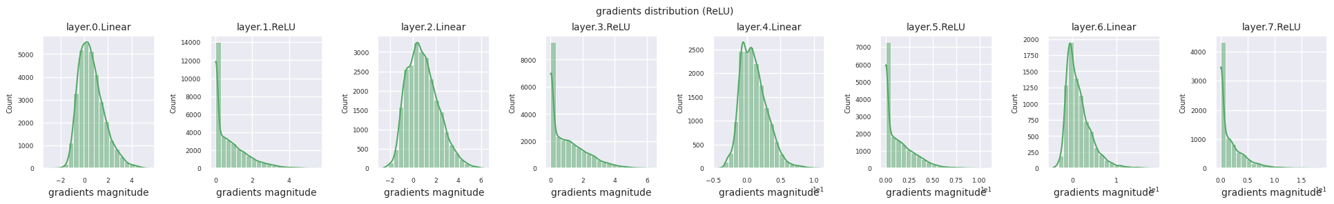
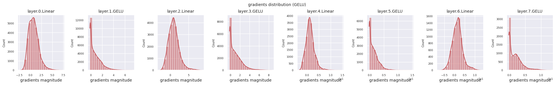
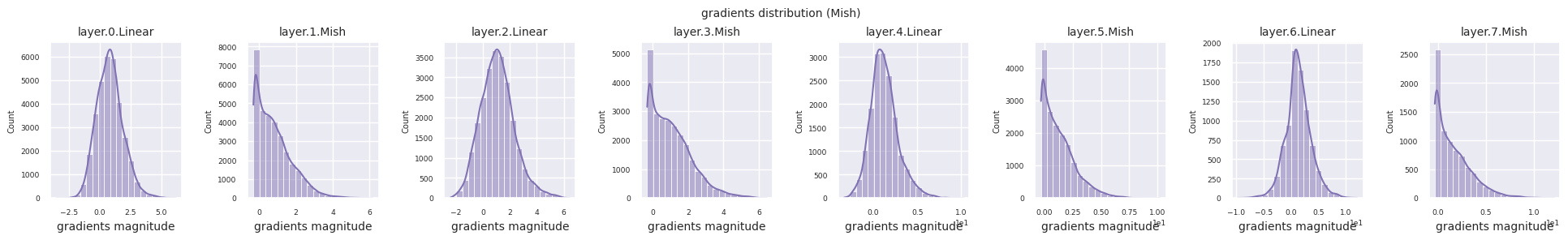
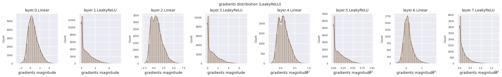
The following code visualizes the gradient distribution of a model using the ReLU activation function.
from dldna.chapter_04.visualization.gradients import visualize_network_gradients

visualize_network_gradients()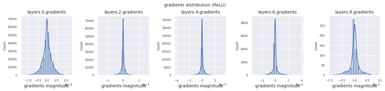
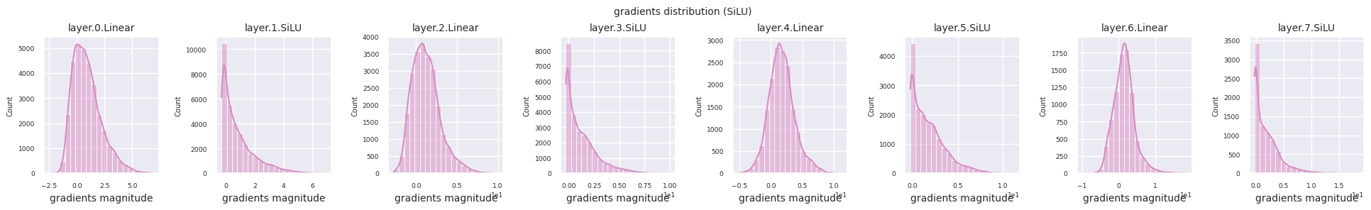
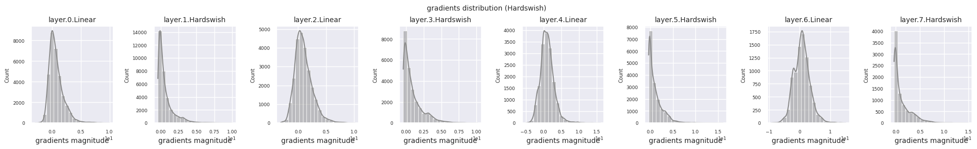
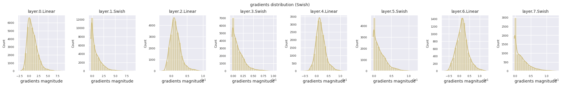
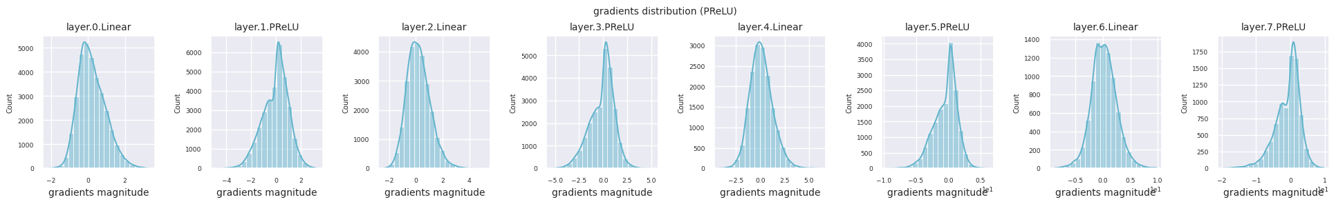
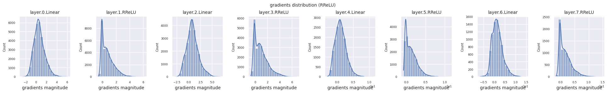
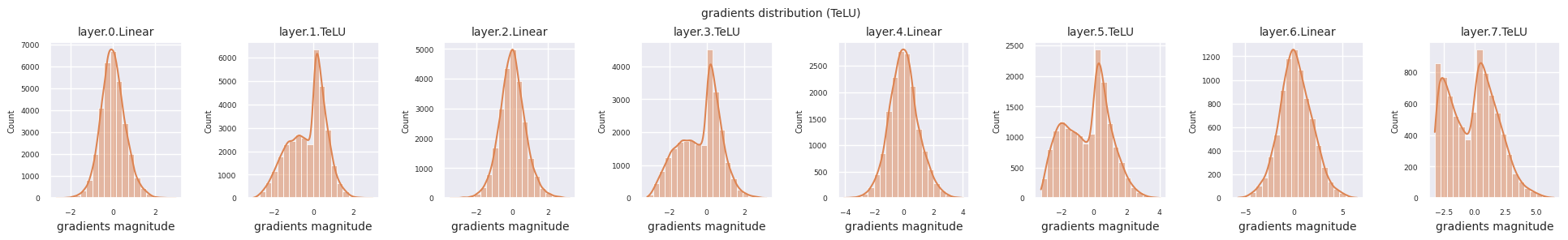
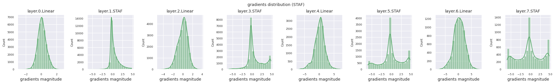
You can analyze the characteristics of the activation function by visualizing the gradient distribution of each layer as a histogram. For ReLU, the output layer shows a gradient value of 10^-2 scale and the input layer shows a gradient value of 10^-3 scale. PyTorch uses He(Kaiming) initialization by default, which is optimized for ReLU series activation functions. Other initialization methods such as Xavier, Orthogonal are also available, and these will be covered in detail in the initialization section.
from dldna.chapter_04.models.activations import act_functions
from dldna.chapter_04.visualization.gradients import get_gradients_weights, visualize_distribution
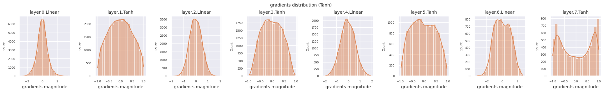
for i, act_func in enumerate(act_functions):
act_func_initiated = act_functions[act_func]()
model = SimpleNetwork(act_func=act_func_initiated).to(device)
gradients, weights = get_gradients_weights(model, train_dataloader)
visualize_distribution(model, gradients, color=f"C{i}")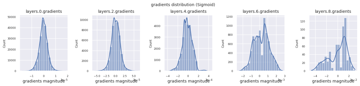

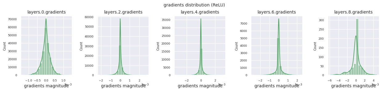
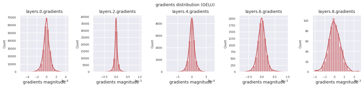
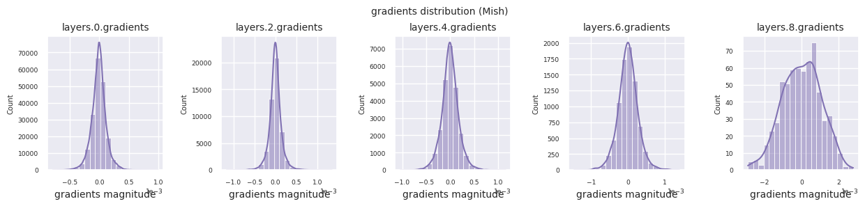
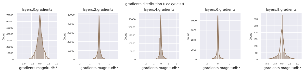
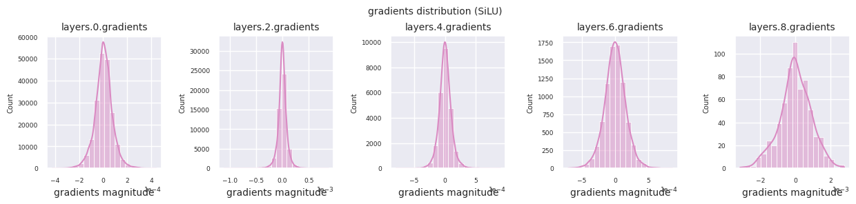
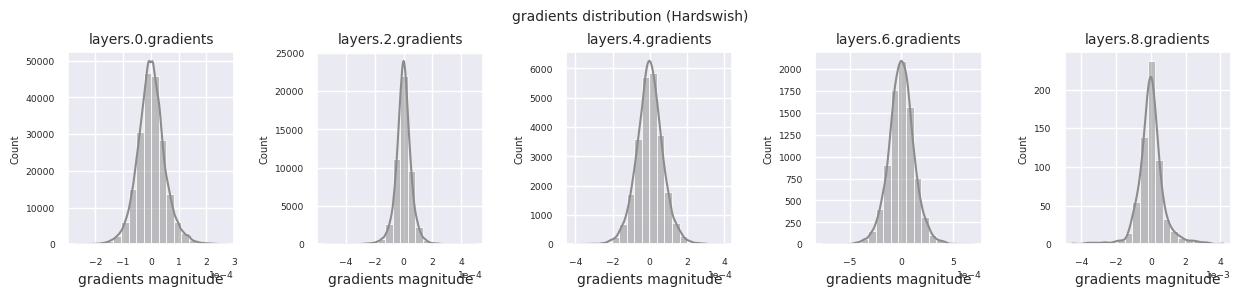
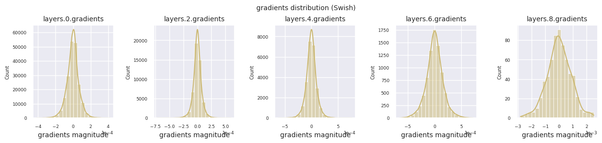
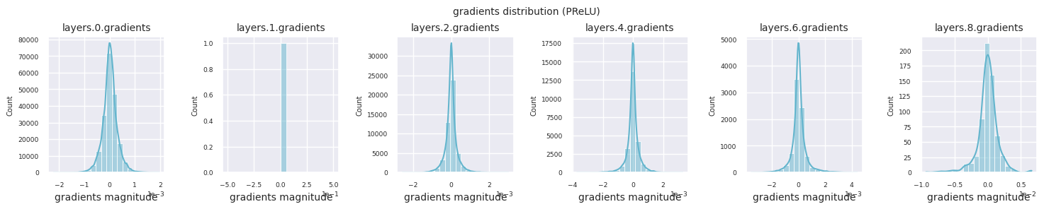
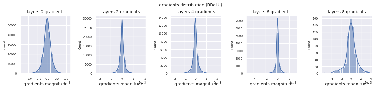
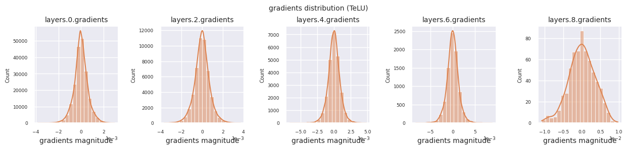
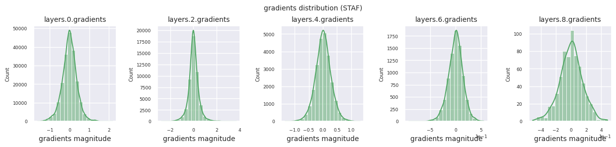
Looking at the gradient distribution by activation function, we can see that Sigmoid shows very small values of \(10^{-5}\) scale from the input layer, which means that the gradient disappearance problem may occur. ReLU has a gradient concentrated around 0, which is due to the characteristic of deactivation (dead neuron) for negative inputs. The latest adaptive activation functions alleviate these problems while maintaining non-linearity. For example, GELU shows a gradient distribution close to a normal distribution, which has a good effect along with batch normalization. Let’s compare it with the case without an activation function.
from dldna.chapter_04.models.base import SimpleNetwork

model_no_act = SimpleNetwork(act_func=nn.ReLU(), no_act = True).to(device)

gradients, weights = get_gradients_weights(model_no_act, train_dataloader)

visualize_distribution(model_no_act, gradients, title="gradients")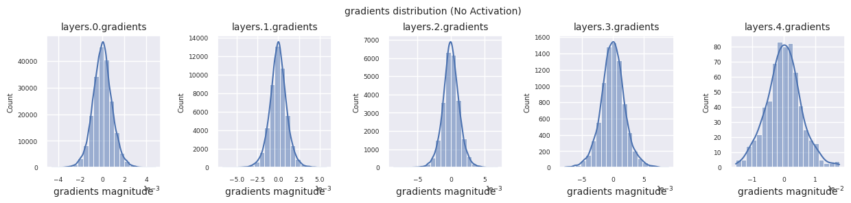
If there is no activation function, the distribution between layers is similar and only the scale changes. This shows that there is no nonlinearity and the feature transformation between layers is limited.
To objectively compare the performance of activation functions, experiments are conducted using the FashionMNIST dataset. As of 2025, there are over 500 activation functions, but in actual deep learning projects, a small number of validated activation functions are mainly used. First, let’s take a look at the basic training process based on ReLU.
import torch.optim as optim
from dldna.chapter_04.experiments.model_training import train_model
from dldna.chapter_04.models.base import SimpleNetwork
from dldna.chapter_04.utils.data import get_device
from dldna.chapter_04.visualization.training import plot_results

model = SimpleNetwork(act_func=nn.ReLU()).to(device)
optimizer = optim.SGD(model.parameters(), lr=1e-2, momentum=0.9)
results = train_model(model, train_dataloader, test_dataloader, device, epochs=10)
plot_results(results)
Starting training for SimpleNetwork-ReLU.Execution completed for SimpleNetwork-ReLU, Execution time = 76.1 secs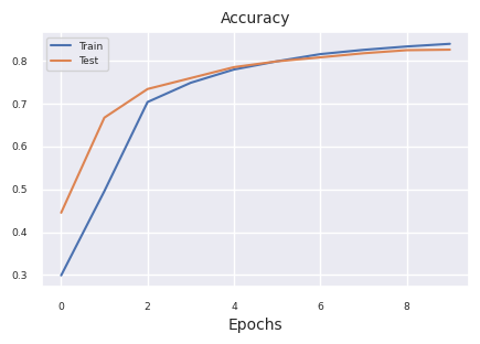
Now we conduct comparative experiments on major activation functions. We keep the composition and training conditions of each model identical to ensure a fair comparison. - 4 hidden layers [256, 192, 128, 64] - SGD optimizer (learning rate=1e-3, momentum=0.9) - Batch size 128 - Trained for 15 epochs
from dldna.chapter_04.experiments.model_training import train_all_models
from dldna.chapter_04.visualization.training import create_results_table


from dldna.chapter_04.experiments.model_training import train_all_models
from dldna.chapter_04.visualization.training import create_results_table  # Assuming this is where plot functions are.

# Train only selected models
# selected_acts = ["ReLU"]  # Select only the desired activation functions
selected_acts = ["Tanh", "ReLU", "Swish"]
# selected_acts = ["Sigmoid", "ReLU", "Swish", "PReLU", "TeLU", "STAF"]
# selected_acts = ["Sigmoid", "Tanh", "ReLU", "GELU", "Mish", "LeakyReLU", "SiLU", "Hardswish", "Swish", "PReLU", "RReLU", "TeLU", "STAF"]
# results_dict = train_all_models(act_functions, train_dataloader, test_dataloader,
#                               device, epochs=15, selected_acts=selected_acts)
results_dict = train_all_models(act_functions, train_dataloader, test_dataloader,
                              device, epochs=15, selected_acts=selected_acts, save_epochs=[1,2,3,4,5,6,7,8,9,10,11,12,13,14,15])

create_results_table(results_dict)
The results came out as shown in the table below. The values will vary depending on each execution environment.
| 모델 | 정확도(%) | 최종 오차(%) | 걸린 시간 (초) |
|---|---|---|---|
| SimpleNetwork-Sigmoid | 10.0 | 2.30 | 115.6 |
| SimpleNetwork-Tanh | 82.3 | 0.50 | 114.3 |
| SimpleNetwork-ReLU | 81.3 | 0.52 | 115.2 |
| SimpleNetwork-GELU | 80.5 | 0.54 | 115.2 |
| SimpleNetwork-Mish | 81.9 | 0.51 | 113.4 |
| SimpleNetwork-LeakyReLU | 80.8 | 0.55 | 114.4 |
| SimpleNetwork-SiLU | 78.3 | 0.59 | 114.3 |
| SimpleNetwork-Hardswish | 76.7 | 0.64 | 114.5 |
| SimpleNetwork-Swish | 78.5 | 0.59 | 116.1 |
| SimpleNetwork-PReLU | 86.0 | 0.40 | 114.9 |
| SimpleNetwork-RReLU | 81.5 | 0.52 | 114.6 |
| SimpleNetwork-TeLU | 86.2 | 0.39 | 119.6 |
| SimpleNetwork-STAF | 85.4 | 0.44 | 270.2 |
Analyzing the experimental results, we can see that
Computational Efficiency: Tanh, ReLU, etc. are the fastest, while STAF is relatively slow due to complex calculations.
Accuracy:
Stability:
These results are comparative under specific conditions, so when selecting an activation function for actual projects, consider the following factors: 1. compatibility with model architecture (e.g., GELU is recommended for transformers) 2. constraints on computational resources (consider Hardswish in mobile environments) 3. characteristics of the task (Tanh is still useful for time series prediction) 4. model size and dataset characteristics
As of 2025, it is standard to use GELU for large language models for computational efficiency, ReLU series for computer vision, and adaptive activation functions for reinforcement learning.
Previously, we examined the distribution of gradient values for each layer in the backpropagation of the initial model. Now, let’s look at what values each layer outputs in the forward calculation using the trained model. Analyzing the output of each layer of the trained model is crucial for understanding the representational power and learning patterns of neural networks. Since the introduction of ReLU in 2010, the problem of dead neurons has become a major consideration in deep neural network design.
First, we visualize the distribution of outputs for each layer in the forward calculation of the trained model.
import os
from dldna.chapter_04.utils.metrics import load_model
from dldna.chapter_04.utils.data import get_data_loaders, get_device
from dldna.chapter_04.visualization.gradients import get_model_outputs, visualize_distribution


device = get_device()
# Re-define the data loaders.
train_dataloader, test_dataloader = get_data_loaders()

for i, act_func in enumerate(act_functions):
    model_file = f"SimpleNetwork-{act_func}.pth"
    model_path = os.path.join("./tmp/models", model_file)

    # Load the model only if the file exists
    if os.path.exists(model_path):
        # Load the model.
        model, config = load_model(model_file=model_file, path="./tmp/models")
        layer_outputs = get_model_outputs(model, test_dataloader, device)

        visualize_distribution(model, layer_outputs, title="gradients", color=f"C{i}")
    else:
        print(f"Model file not found: {model_file}")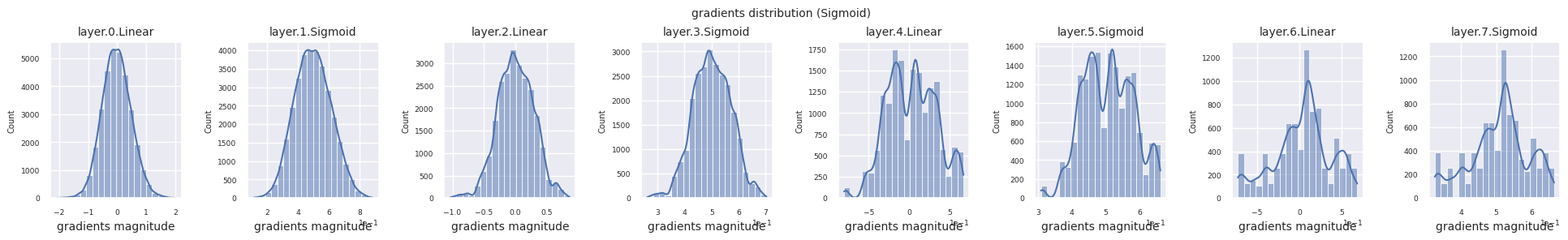
Dead neurons (inactive neurons) refer to neurons that always output 0 for all inputs. This is a particularly important issue in the ReLU family of activation functions. To find dead neurons, one can pass all training data through them and check if they always output 0. This can be done by taking the output values for each layer and using logical operations to mask when they are always 0.
# 3 samples (1 batch), 5 columns (each a neuron's output). Columns 1 and 3 always show 0.
batch_1 = torch.tensor([[0, 1.5, 0, 1, 1],
                        [0, 0,  0, 0, 1],
                        [0, 1,  0, 1.2, 1]])

# Column 3 always shows 0
batch_2 = torch.tensor([[1.1, 1, 0, 1, 1],
                        [1,   0, 0, 0, 1],
                        [0,   1, 0, 1, 1]])

print(batch_1)
print(batch_2)

# Use the .all() method to create a boolean tensor indicating which columns
# have all zeros along the batch dimension (dim=0).
batch_1_all_zeros = (batch_1 == 0).all(dim=0)
batch_2_all_zeros = (batch_2 == 0).all(dim=0)

print(batch_1_all_zeros)
print(batch_2_all_zeros)

# Declare a masked_array that can be compared across the entire batch.
# Initialized to all True.
masked_array = torch.ones(5, dtype=torch.bool)
print(f"masked_array = {masked_array}")

# Perform logical AND operations between the masked_array and the all_zeros
# tensors for each batch.
masked_array = torch.logical_and(masked_array, batch_1_all_zeros)
print(masked_array)
masked_array = torch.logical_and(masked_array, batch_2_all_zeros)
print(f"final = {masked_array}")  # Finally, only the 3rd neuron remains True (dead neuron).
tensor([[0.0000, 1.5000, 0.0000, 1.0000, 1.0000],
[0.0000, 0.0000, 0.0000, 0.0000, 1.0000],
[0.0000, 1.0000, 0.0000, 1.2000, 1.0000]])
tensor([[1.1000, 1.0000, 0.0000, 1.0000, 1.0000],
[1.0000, 0.0000, 0.0000, 0.0000, 1.0000],
[0.0000, 1.0000, 0.0000, 1.0000, 1.0000]])
tensor([ True, False, True, False, False])
tensor([False, False, True, False, False])
masked_array = tensor([True, True, True, True, True])
tensor([ True, False, True, False, False])
final = tensor([False, False, True, False, False])The function to calculate disabled neurons is calculate_disabled_neuron. It is in visualization/training.py. Let’s analyze the ratio of disabled neurons in the actual model.
from dldna.chapter_04.visualization.training import calculate_disabled_neuron
from dldna.chapter_04.models.base import SimpleNetwork

# Find in the trained model.
model, _ = load_model(model_file="SimpleNetwork-ReLU.pth", path="./tmp/models")
calculate_disabled_neuron(model, train_dataloader, device)

model, _ = load_model(model_file="SimpleNetwork-Swish.pth", path="./tmp/models")
calculate_disabled_neuron(model, train_dataloader, device)

# Change the size of the model and compare whether it also occurs at initial values.
big_model = SimpleNetwork(act_func=nn.ReLU(), hidden_shape=[2048, 1024, 1024, 512, 512, 256, 128]).to(device)
calculate_disabled_neuron(big_model, train_dataloader, device)
Number of layers to compare = 4Number of disabled neurons (ReLU) : [0, 6, 13, 5]
Ratio of disabled neurons = 0.0%
Ratio of disabled neurons = 3.1%
Ratio of disabled neurons = 10.2%
Ratio of disabled neurons = 7.8%
Number of layers to compare = 4Number of disabled neurons (Swish) : [0, 0, 0, 0]
Ratio of disabled neurons = 0.0%
Ratio of disabled neurons = 0.0%
Ratio of disabled neurons = 0.0%
Ratio of disabled neurons = 0.0%
Number of layers to compare = 7Number of disabled neurons (ReLU) : [0, 0, 6, 15, 113, 102, 58]
Ratio of disabled neurons = 0.0%
Ratio of disabled neurons = 0.0%
Ratio of disabled neurons = 0.6%
Ratio of disabled neurons = 2.9%
Ratio of disabled neurons = 22.1%
Ratio of disabled neurons = 39.8%
Ratio of disabled neurons = 45.3%According to current research results, the severity of the dying neuron problem varies depending on the depth and width of the model. Notably, 1. As the model deepens, the proportion of inactive neurons in ReLU increases sharply 2. Adaptive activation functions (STAF, TeLU) effectively alleviate this problem 3. In Transformer architectures, GELU greatly reduces the dying neuron problem 4. In the latest MoE (Mixture of Experts) models, the problem is solved by using different activation functions for each expert network
Therefore, when designing neural networks with many layers, alternatives such as GELU, STAF, and TeLU should be considered instead of ReLU, and especially for ultra-large models, a choice that considers both computational efficiency and the dying neuron problem is necessary.
The selection of activation functions is one of the crucial decision-making factors in neural network design. Activation functions directly influence the network’s ability to learn complex patterns, training speed, and overall performance. The following outlines the latest research findings and best practices organized by application domain.
The following provides a more systematic approach to selecting activation function candidates:
Recent Key Trends and Considerations:
Most importantly, always experiment! Start with reasonable defaults (GELU or ReLU/LeakyReLU), but be prepared to try other options if you don’t achieve desired performance. Small experiments that change the activation function alone, while keeping other hyperparameters constant, are essential for making informed choices.
Activation functions are one of the core components of deep learning models, significantly influencing the model’s expressiveness, learning speed, and final performance. In addition to existing widely used activation functions (ReLU, GELU, Swish, etc.), numerous researchers have proposed new activation functions. This deep dive explores the process of designing your own activation function step by step and learns how to implement and test it using PyTorch.
Before designing a new activation function, let’s recall the conditions for an “ideal” activation function described in section 4.2.
Additionally, consider the following aspects:
The most common method for designing new activation functions is by combining or modifying existing ones.
If a new activation function is proposed, a mathematical analysis must be performed.
An activation function validated by mathematical analysis can be easily implemented using PyTorch. A new class that inherits torch.nn.Module is created, and the operation of the activation function is defined in the forward method. If necessary, learnable parameters can be defined as torch.nn.Parameter.
Example: Implementation of “SwiGELU” Activation Function
Let’s propose a new activation function “SwiGELU” that combines Swish and GELU and implement it using PyTorch.
import torch
import torch.nn as nn
import torch.nn.functional as F

class SwiGELU(nn.Module):
    def __init__(self):
        super().__init__()

    def forward(self, x):
        return 0.5 * (x * torch.sigmoid(x) + F.gelu(x))
Description:
SwiGELU(x) = 0.5 * (x * sigmoid(x) + GELU(x))If a new activation function is proposed, an experiment should be conducted to compare its performance with existing activation functions using benchmark datasets (e.g., CIFAR-10, CIFAR-100, ImageNet).
train_model_with_metrics functioncalculate_disabled_neuron functionIf the experimental results are good, it’s a good idea to theoretically analyze why the new activation function performs well. * Loss Landscape Analysis: Analyzes the impact of activation functions on the loss function space (loss landscape). (Refer to Section 4.2 Deep Dive) * Neural Tangent Kernel (NTK) Analysis: Analyzes the role of activation functions in infinitely wide neural networks. * Fokker-Planck Equation: Analyzes the dynamic characteristics of activation functions. (Refer to research on Swish)
Designing and evaluating new activation functions is not an easy task, but it is a promising research area that can improve the performance of deep learning models. Overcoming the limitations of existing activation functions and finding activation functions more suitable for specific problems or architectures is one of the important tasks in deep learning research. We hope that the step-by-step approach presented in this deep dive, PyTorch implementation examples, and experimental and analytical guidelines will help you design your own activation function.
Introduction:
ReLU, GELU, and other fixed activation functions are widely used in deep learning models but may not be optimal for specific problems or data distributions. Recently, research has been actively conducted to adjust the activation function adaptively according to the data or task. In this deep dive, we explore the potential of adaptive activation functions and future research directions.
Adaptive activation functions can be broadly classified as follows:
Parametric Adaptation: Introduce learnable parameters into the activation function to adjust its shape according to the data.
Structural Adaptation: Combine multiple basis functions or change the network structure to dynamically construct the activation function.
Input-based Adaptation: Change or mix the activation function based on the characteristics of the input data.
Idea: Define multiple “expert” activation functions and dynamically determine their weights for each input data.
Mathematical Expression:
\(f(x) = \sum_{k=1}^K g_k(x) \cdot \phi_k(x)\)
Research Tasks:
| Research Direction | Description |
|---|---|
| Parametric Adaptation | Adjusting the shape of the activation function using learnable parameters |
| Structural Adaptation | Dynamically constructing the activation function by combining multiple basis functions or changing the network structure |
| Input-based Adaptation | Changing or mixing the activation function based on the characteristics of the input data |
| Mixture of Experts (MoE) | Defining multiple expert activation functions and dynamically determining their weights for each input data |
Idea: Utilize domain knowledge from physics, biology, etc. to impose constraints or prior knowledge on the design of activation functions.
Examples:
Research Tasks:
Adaptive activation functions are a promising research area that can improve the performance of deep learning models. However, the following tasks remain:
In future research, it is essential to develop adaptive activation functions that are more efficient, interpretable, and have better generalization performance while addressing these challenges.
Write the formulas for Sigmoid, Tanh, ReLU, Leaky ReLU, GELU, and Swish functions and draw their graphs using matplotlib or Desmos.
Find the derivatives (differential) of each activation function and draw their graphs.
Train a neural network composed only of linear transformations without activation functions using the FashionMNIST dataset, and measure its test accuracy. (Use the SimpleNetwork implemented in Chapter 1)
Compare the results obtained from problem 3 with those of a neural network using the ReLU activation function and explain the role of activation functions.
Implement PReLU, TeLU, and STAF activation functions in PyTorch (inherit from nn.Module).
forward method. If necessary, define learnable parameters using nn.Parameter.Train a neural network that includes the previously implemented activation functions using the FashionMNIST dataset and compare their test accuracies.
For each activation function, visualize the distribution of gradients during training and measure the ratio of “dead neurons”. (Use functions implemented in Chapter 1)
Investigate methods to alleviate the “dead neuron” problem and explain their principles. (Leaky ReLU, PReLU, ELU, SELU, etc.)
Implement the Rational activation function in PyTorch and explain its characteristics and pros and cons.
Implement B-spline or Fourier-based activation functions in PyTorch and explain their characteristics and pros and cons.
Propose a new activation function of your own and evaluate its performance compared to existing activation functions (with experimental results and theoretical justification).
Formulas and graphs of Sigmoid, Tanh, ReLU, Leaky ReLU, GELU, Swish functions:
| Activation Function | Formula | Graph (Reference) |
|---|---|---|
| Sigmoid | \(\sigma(x) = \frac{1}{1 + e^{-x}}\) | Sigmoid |
| Tanh | \(tanh(x) = \frac{e^{x} - e^{-x}}{e^{x} + e^{-x}}\) | Tanh |
| ReLU | \(ReLU(x) = max(0, x)\) | ReLU |
| Leaky ReLU | \(LeakyReLU(x) = max(ax, x)\) , (\(a\) is a small constant, usually 0.01) | (Leaky ReLU has a small slope(\(a\)) in the part where x < 0 of the ReLU graph) |
| GELU | \(GELU(x) = x\Phi(x)\) , (\(\Phi(x)\) is the Gaussian cumulative distribution function) | GELU |
| Swish | \(Swish(x) = x \cdot sigmoid(\beta x)\) , (\(\beta\) is a constant or learning parameter) | Swish |
Derivatives of each activation function: | Activation Function | Derivative | | :———- | :—————————————————————————————— | | Sigmoid | \(\sigma'(x) = \sigma(x)(1 - \sigma(x))\) | | Tanh | \(tanh'(x) = 1 - tanh^2(x)\) | | ReLU | \(ReLU'(x) = \begin{cases} 0, & x < 0 \\ 1, & x > 0 \end{cases}\) | | Leaky ReLU | \(LeakyReLU'(x) = \begin{cases} a, & x < 0 \\ 1, & x > 0 \end{cases}\) | | GELU | \(GELU'(x) = \Phi(x) + x\phi(x)\), (\(\phi(x)\) is the Gaussian probability density function) | | Swish | \(Swish'(x) = sigmoid(\beta x) + x \cdot sigmoid(\beta x)(1 - sigmoid(\beta x))\beta\) |
FashionMNIST, Training and Accuracy Measurement of Neural Network without Activation Function:
Comparison with ReLU Activation Function and Explanation of its Role:
PReLU, TeLU, STAF PyTorch Implementation:
import torch
import torch.nn as nn

class PReLU(nn.Module):
    def __init__(self, num_parameters=1, init=0.25):
        super().__init__()
        self.alpha = nn.Parameter(torch.full((num_parameters,), init))

    def forward(self, x):
        return torch.max(torch.zeros_like(x), x) + self.alpha * torch.min(torch.zeros_like(x), x)
class TeLU(nn.Module): def init(self, alpha=1.0): super().__init__() self.alpha = nn.Parameter(torch.tensor(alpha))
def forward(self, x): return torch.where(x > 0, x, self.alpha * (torch.exp(x) - 1))
class STAF(nn.Module): def init(self, tau=25): super().__init__() self.tau = tau self.C = nn.Parameter(torch.randn(tau)) self.Omega = nn.Parameter(torch.randn(tau)) self.Phi = nn.Parameter(torch.randn(tau))
def forward(self, x):
    result = torch.zeros_like(x)
    for i in range(self.tau):
        result += self.C[i] * torch.sin(self.Omega[i] * x + self.Phi[i])
    return result
FashionMNIST, Activation Function Comparison Experiment:
Gradient Distribution Visualization, “Dead Neuron” Ratio Measurement:
Methods and Principles to Alleviate the “Dead Neuron” Problem:
Rational Activation Function PyTorch Implementation, Characteristics, and Advantages/Disadvantages:
import torch
import torch.nn as nn

class Rational(nn.Module):
    def __init__(self, numerator_coeffs, denominator_coeffs):
        super().__init__()
        self.numerator_coeffs = nn.Parameter(numerator_coeffs)
        self.denominator_coeffs = nn.Parameter(denominator_coeffs)
def forward(self, x): numerator = torch.polyval(self.numerator_coeffs, x) # polynomial calculation denominator = 1 + torch.polyval(self.denominator_coeffs, torch.abs(x)) # absolute value and polynomial return numerator / denominator
B-spline or Fourier-based activation function PyTorch implementation, characteristics, and advantages/disadvantages:
B-spline activation function:
import torch
import torch.nn as nn
from scipy.interpolate import BSpline
import numpy as np

class BSplineActivation(nn.Module):
    def __init__(self, knots, degree=3):
        super().__init__()
        self.knots = knots
        self.degree = degree
        self.coeffs = nn.Parameter(torch.randn(len(knots) + degree - 1)) # control points

    def forward(self, x):
        # B-Spline calculation
        b = BSpline(self.knots, self.coeffs.detach().numpy(), self.degree) # separate coefficients
        spline_values = torch.tensor(b(x.detach().numpy()), dtype=torch.float32) # input x into B-Spline
        return spline_values * self.coeffs.mean() # detach, numpy() or error
         # detach, numpy() or error
Characteristics: Locally controlled flexible curve. Shape adjusted by knots and degree.
Advantages: Smooth function expression. Local feature learning.
Disadvantages: Performance affected by knot setting. Increased computational complexity.
Proposal of a new activation function and performance evaluation:
```python
import torch
import torch.nn as nn
import torch.nn.functional as F
class SwiGELU(nn.Module): # Swish + GELU
  def forward(self, x):
    return 0.5 * (x * torch.sigmoid(x) + F.gelu(x))
```

SwiGELU combines the smoothness of Swish and the regularization effect of GELU.